Reprinted from New Machine Vision

1、 Background

For autonomous driving, mapping is essential. Currently, mainstream manufacturers are preparing for the transition from HD to "map free" technology. However, there is still a long way to go to achieve true "map free" technology. For mapping, it includes many road elements such as lane markings, stop lines, zebra crossings, diversion properties, road edges, and centerlines (including guide lines). Here, the prediction of the centerline is usually based on the trajectory and fitted through mathematical formulas. Currently, models are gradually being used for prediction in academia. However, for downstream (PNC), there are still issues such as insufficient smoothness and inaccurate curvature. However, this is not within the scope of this plan discussion and will be ignored for now. You can write about it when you have time in the future. Road boundaries are also crucial for PNC, constraining the vehicle's driving range and avoiding physical collisions. There are usually several methods for generating road boundaries. One is to use them as part of the lane lines and output them along with the model. However, there are no obvious features of the lane lines, making it easy to miss detection. Moreover, the road boundaries are irregular, and the segmentation based approach is more stable than the anchor based approach. Another method is HD, which creates virtual roadside boundaries based on distance and rules based on the processed lane markings. This article presents a new solution that is slightly cumbersome, but the advantage is that it can be processed and generated using existing public datasets for quick validation. The disadvantage is that this solution does not have timeliness and is an offline method.

2、 Plan

The pipeline of the entire scheme for the dataset and model is shown in the above figure. In order to quickly verify the effect, the publicly available dataset BDD100k was directly used. This dataset is mainly used for driving areas, lane lines, and panoramic segmentation. Its lane markings have marked edges, but there is no distinction between categories, so it cannot be directly used, so freespace is used for verification. In terms of model, theoretically any segmentation can be used. YOLOPv2 is used here, and the model provides trained weights and inference scripts. The output is shown below.

YOLOPv2 output

There is an issue with the difference between this dataset and the requirements for mapping. As mentioned earlier, this solution is based on freespace, but freespace is distinguished by the actual visible boundary rather than the road boundary, so there is some difference from the actual mapping requirements. The green one shown in the above figure is the result of freespace, which is blocked by the road boundary by the left car. Therefore, freespace will use the vehicle boundary as its own boundary. If it is real-time, there is no problem, but if it is offline, it will generate a diff. If there are cars on the first day, and after creating the map, it is found that there are no cars on the second day, then the range of available traffic will be squeezed. So if it is actually used in the future, the boundary of the road needs to be used as the boundary line of the freespace.

overview

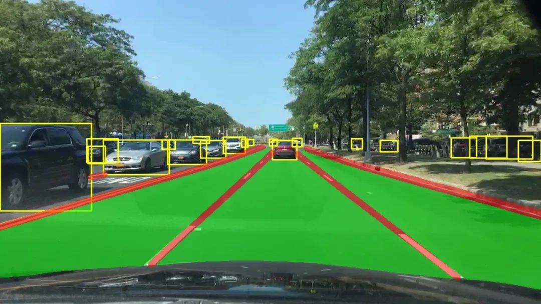
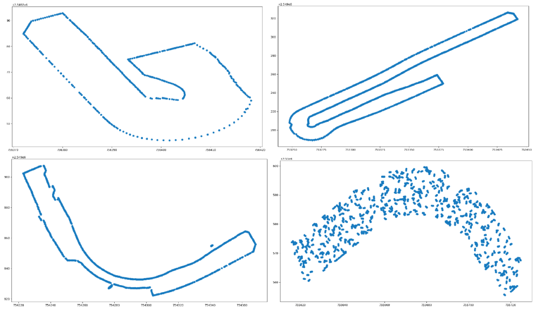
The overall scheme of the entire scheme is shown above. After distortion correction is applied to the images obtained from the front view camera, the model is fed and the corresponding freespace is output. Due to the poor projection effect of IPM on boundaries and distant areas, only a range of 15m in front of the vehicle and 20m on the left and right sides is selected. The obtained freespace is projected onto the world coordinate system based on the internal and external parameters and the vehicle position. By stacking consecutive frames, a 2D point cloud in the world coordinate system can be generated. In fact, what is needed is the edge, so it is necessary to process the point cloud to obtain the edge of the road. Here, we have tried point cloud processing methods such as PCL and AlphaShape, which can solve the extraction of some cases. However, it still depends on parameter tuning and cannot be automated. Below are some bad case examples.

2D point cloud in world coordinate system

2D point cloud

PCL

PCL filtering+edge extraction results

AlphaShape

Alphashape extraction results

To address the above issue, first project and map the point cloud of the world coordinate system. Here, I set 1 pixel to represent 0.05m, as a lane line is approximately 15-20cm wide, so this slight error does not affect the result of back projection. After mapping, the point cloud of the grid can be obtained. Due to the divergence of distant points during the conversion from UV to world coordinate system, it is necessary to filter and fill them in the grid image, as shown in the following figure before and after processing.

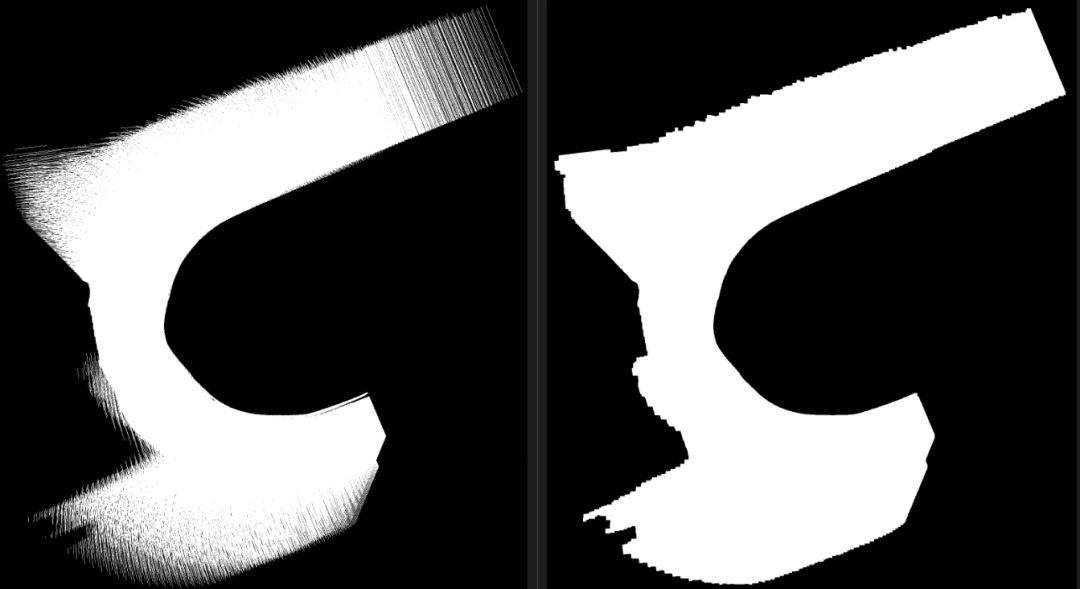
Grid processing

Then, image processing methods can be used to obtain the edges of the entire raster image and backproject it onto the world coordinate system based on the mapping relationship. The vectorized points can be sparsely sampled or interpolated according to downstream requirements, and the results are shown below.

Edge processing

The next step is to truncate the two ends of the edge based on RTK information (otherwise, the closed area will not be driven by vehicles). This step is slightly cumbersome, and the logic is simplified as follows:

Determine whether it is a straight, turning, or turning intersection based on attributes

Set different segmentation logic based on different attributes

Straight | Turn, using double headed segmentation, based on the starting and ending RTK positions, by setting distance parameters to find the segmentation points on the left and right ends for segmentation.

Turn around, use single head segmentation, select the starting position and locate the key points. By setting a longer distance to run through the entire turning intersection, locate 4 points for segmentation.

Filter outliers and smooth them out.

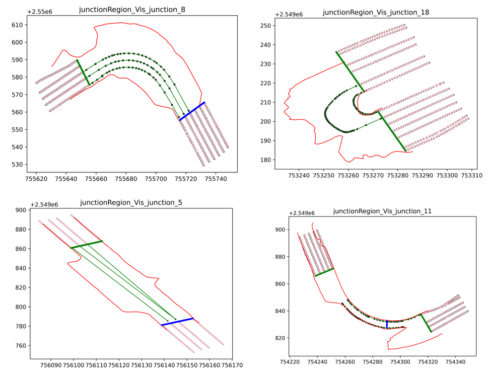
The effect before and after splitting, where blue represents the edge after splitting

Finally, it's about constantly optimizing and iterating the logic. If the model's performance is not good, then optimize the model. If the logic is not good enough, then optimize the logic. Previously, it was mentioned that the freespace in the dataset is not distinguished by the actual road edge boundaries, so model optimization will need to be carried out on the benchmark data later.

To verify if the accuracy is high enough, it can be spliced onto HD for comparison

The bottom map shows the lane lines and reference lines provided by HD, with red indicating the road boundary at the intersection

In the end, PNC cannot actually use such irregular edges. It has been proven that everything still needs to be aligned with HD, so quadratic constraints need to be applied to optimize curve smoothing based on the generated edges. I won't go into detail here, it's another very complex mathematical problem.

Optimization effect based on edge constraints

3、 Conclusion

This plan only provides a quick implementation approach, but there are actually many details that need to be optimized. However, compared to the scheme that only predicts road edges, the freespace based scheme has a relatively stronger generalization ability and can annotate data for multiple purposes. However, in terms of speed, it should be noted that offline can meet the requirements, while online real-time still depends on the efficiency of optimization.