Sensor calibration is a basic requirement for autonomous driving. A vehicle is equipped with multiple sensors, and their coordinate relationships need to be determined. The co founder and CTO of the Bay Area autonomous driving startup ZooX are Jesse Levinson, a student of Sebastia Thrun, whose doctoral thesis is sensor calibration.
This work can be divided into two parts: internal parameter calibration and external parameter calibration. The internal parameter determines the mapping relationship inside the sensor, such as the focal length of the camera, eccentricity, and pixel aspect ratio (+distortion coefficient), while the external parameter determines the transformation relationship between the sensor and an external coordinate system, such as attitude parameters (rotation and translational 6 degrees of freedom).
Camera calibration used to be a prerequisite for 3D reconstruction in computer vision. Zhang Zhengyou's famous Zhang calibration method, which uses Absolute Conic invariance to obtain a plane calibration algorithm, simplifies the control field.
The emphasis here is to discuss the external parameter calibration between different sensors, especially the calibration between the laser radar and the camera.
In addition, calibration between GPS/IMU and camera or LiDAR, as well as calibration between radar and camera, is also common in the development of autonomous driving. The biggest problem of calibration between different sensors is how to measure the best, because the data types obtained are different:
The camera is a pixel array of RGB images;
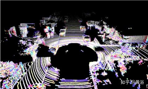
Lidar is a 3D point cloud distance information (possibly with grayscale values of reflection);
GPS-IMU provides vehicle position and attitude information;
The radar is a 2-D reflection map.
In this way, the objective function to minimize the calibration error will be different for different sensor pairs.
In addition, there are two calibration methods: targetless and target. The former is performed in a natural environment with fewer constraints and does not require the use of specialized targets; The latter requires a dedicated control field with a ground truth target, such as a typical checkerboard flat panel.
Here, we will only discuss the targetless method and provide several calibration algorithms in sequence.
Firstly, hand eye calibration
This is a problem that is widely studied by calibration methods under certain constraints: it can be broadly understood that a "hand" (such as GPS/IMU) and an "eye" (LiDAR/camera) are both fixed on the same machine. Therefore, when the machine moves, the attitude changes of the "hand" and "eye" must satisfy certain constraint relationships. By solving an equation, the coordinate transformation relationship between the "hand" and "eye" can be obtained, which is generally in the form of AX=XB.
There are two types of hand eye systems: eye in hand and eye to hand. Here, we clearly refer to the former, which means that both hands and eyes are in motion.
Hand eye calibration can be divided into two-step and single-step methods, with the most famous paper being "Hand eye calibration using dual quantization". It is generally believed that the single-step method has higher accuracy than the two-step method, with the former estimating rotation and then translation.
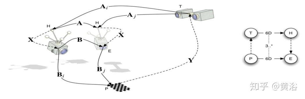
Here, let's take a look at the calibration algorithms for LiDAR and Camera through the paper "LiDAR and Camera Calibration Using Motion Estimated by Sensor Fusion Odometry" by the University of Tokyo.
Obviously, it is an extended problem for solving hand eye calibration, namely 2D-3D calibration, as shown in the figure:

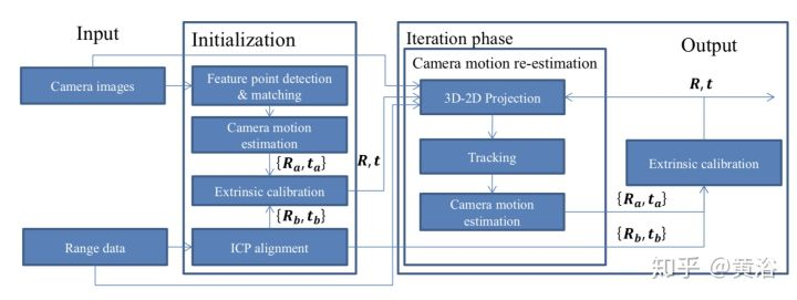
ICP is used to solve the attitude changes of the LiDAR, while feature matching is used for the motion of the camera. The latter has a scale problem with monocular SFM, and the paper proposes a solution based on sensor fusion: the initial estimation comes from scale-free camera motion and scaled LiDAR motion; Afterwards, the motion of the scale camera will be re estimated with the addition of LiDAR point cloud data. The external parameters of the last two can be obtained through hand eye calibration. The following diagram is the algorithm flowchart:
The typical solution for hand eye calibration is a two-step method: first, solve the rotation matrix, and then estimate the translation vector. The formula is given below:
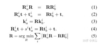
Due to the scale issue, the above solution is unstable, so we need to use the data from LiDAR to create an article, as shown in the following figure:
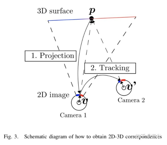
The points of a 3D point cloud are tracked in the image, and their 2D-3D correspondence can be described as follows:
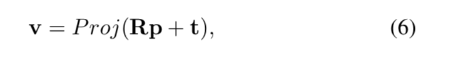
And the problem solved becomes:
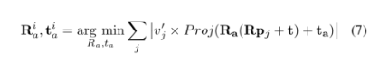
The initial solution of the optimization problem above was obtained through the classical P3P method.
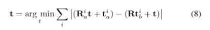
After obtaining the motion parameters of the camera, the rotation and translation 6 parameters can be obtained in the two-step hand eye calibration method, where the translation estimation is as follows:
Note: Here, estimating camera motion and estimating hand eye calibration are performed alternately to improve estimation accuracy. In addition, the author also found some strategies for camera motion to affect calibration accuracy, as analyzed in the following figure:
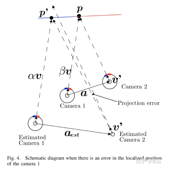
It can be summarized that: 1) the smaller the actual movement of the camera a, the smaller the projection error; 2) The smaller the (), the smaller the projection error. The first point indicates that the camera movement should be small during calibration, and the second point indicates that the depth of the surrounding environment during calibration should change less, such as walls.
In addition, it was found that increasing the rotation angle of camera motion reduces the error propagation from camera motion estimation to hand eye calibration.
This method cannot be used in outdoor natural environments because it is difficult to determine the image points projected by point clouds.
There are three papers on how to optimize LiDAR camera calibration, which do not estimate calibration parameters based on the matching error between the 3D point cloud and image points, but directly calculate the depth map formed by the point cloud in the image plane, which has a global matching measurement with the image obtained by the camera.
However, these methods require a lot of iteration, and the best approach is to generate initial values based on hand eye calibration.
In addition, the University of Michigan has adopted lidar reflection values, while the University of Sydney has improved upon them. Both methods are not as convenient as Stanford University's, and calibration is directly achieved through point cloud and image matching.
Stanford Thesis“Automatic Online Calibration of Cameras and Lasers”。
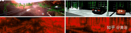
Stanford's method is to adjust the drift of the calibration online, as shown in the following figure: Accurate calibration should match the green points (depth discontinuity) and red edges (through inverse distance transformation (IDT)) in the graph.
The objective function for calibration is defined as follows:
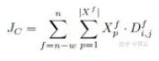
Where w is the video window size, f is frame #, (i, j) is the pixel position in the image, and p is the 3D point of the point cloud. X represents the LiDAR point cloud data, and D is the result of the image undergoing IDT.
The following is an example of the results of real-time online calibration:
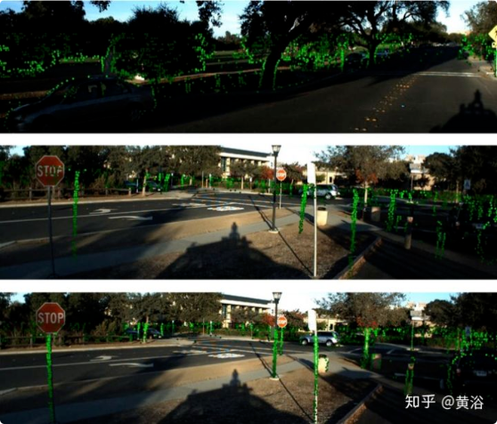
The first line is calibrated, the second line shows drift, and the third line is recalibrated.
A paper from the University of Michigan “Automatic Targetless Extrinsic Calibration of a 3D Lidar and Camera by Maximizing Mutual Information”。
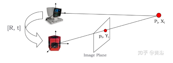
The calibration task is defined here as solving the conversion relationship between two sensors, as shown in the figure: solving R, T.
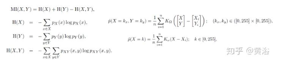
The defined Mutual Information (MI) objective function is an entropy value:
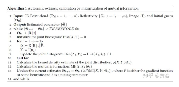
The algorithm used for solving is the gradient method:
The following image is an example of calibration: RGB pixel and point cloud calibration.
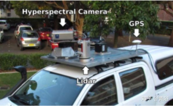
Thesis from the University of Sydney, Australia “Automatic Calibration of Lidar and Camera Images using Normalized Mutual Information”。
This article is an improvement on the above method. The sensor configuration is shown in the figure:
The calibration process is shown in the following figure:
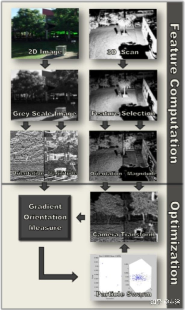
A new measure, Gradient Orientation Measure (GOM), is defined as follows:
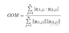
In fact, it is a gradient correlation measure between images and LiDAR point clouds.
When matching point cloud data with image data, it is necessary to project the point cloud onto a cylindrical image, as shown in the figure:
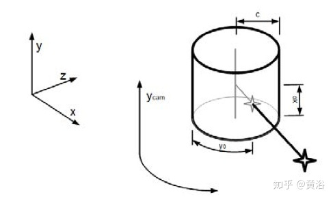
The projection formula is as follows:
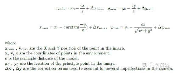
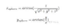
Before calculating the gradient of a point cloud, it is necessary to project the point cloud onto a sphere. The formula is as follows:
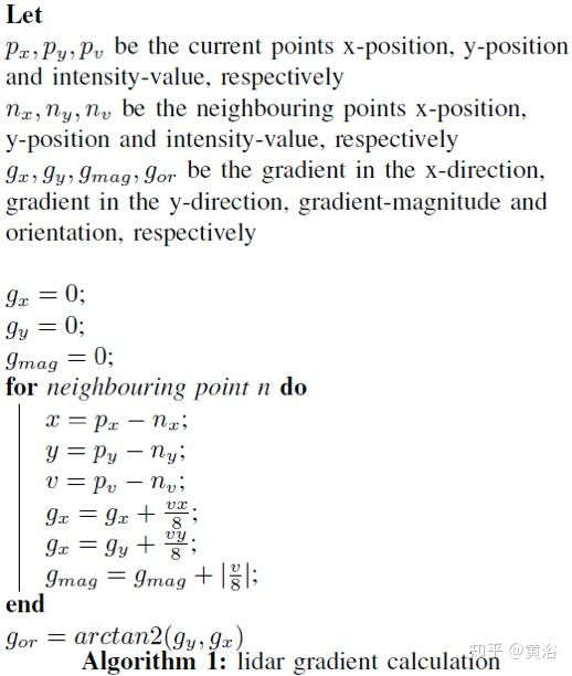
Finally, the gradient calculation method for point clouds is as follows:
The task of calibration is to solve for the maximum GOM, and the Monte Carlo method, similar to particle filter, was used in the article. The following figure is an example of a result:
2 IMU camera calibration
German Fraunhofer paper "INS Camera Calibration without Ground Control Points".
Although this article is for the calibration of drones, it is also suitable for vehicles.
This is the East, North, Up (ENU) coordinate system defined by IMU:
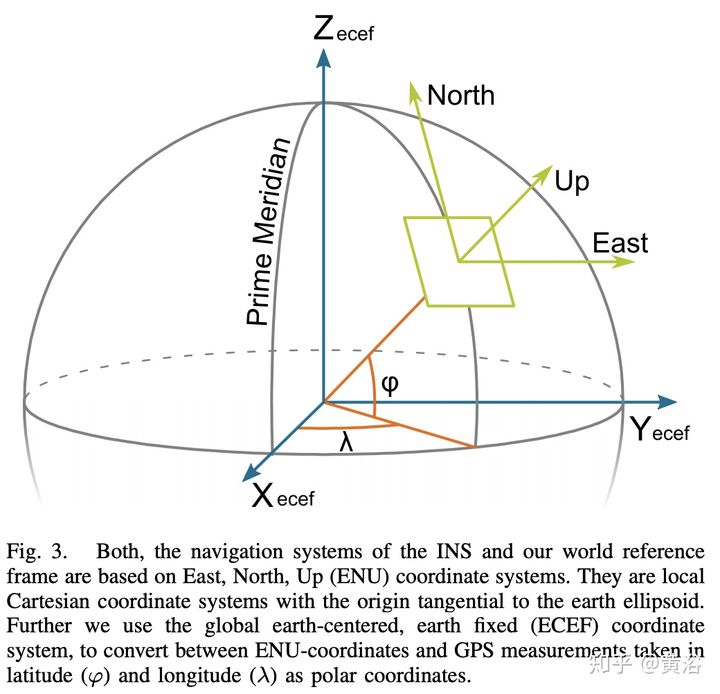
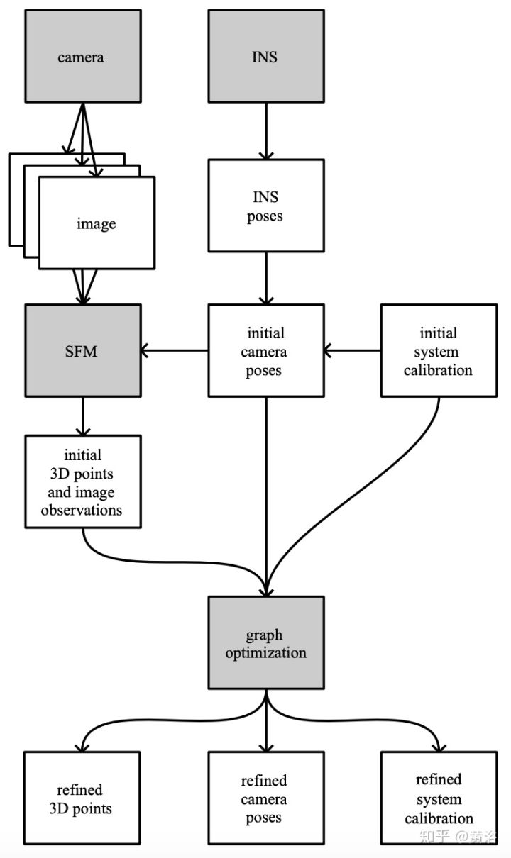
In fact, IMU camera calibration and LiDAR camera calibration are similar, first solving a hand eye calibration, and then optimizing the results. It's just that IMU doesn't have any feedback information available, only attitude data, so we did pose graph optimization. The following diagram is a flowchart: the camera still uses SFM to estimate the pose.
This is the image calibration board used:

3. Calibration of LiDAR system
Oxford University Thesis “Automatic self-calibration of a full field-of-view 3D n-laser scanner".
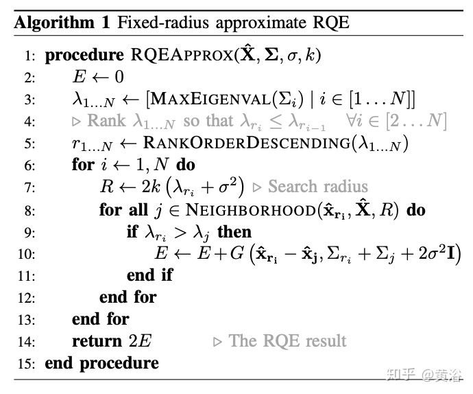
This article defines the "crisis" of point clouds as a quality measure, which is obtained through an entropy function Re ́ Minimizing nyi Quadratic Entropy (RQE) as the optimization objective for online calibration of LiDAR. (Note: The author also discussed solutions to the clock bias problem of LiDAR.)
"Crisp" actually describes the point cloud distribution as a density in the form of a Gaussian Mixture Model (GMM). According to the definition of information entropy, RQE is chosen as the measure:

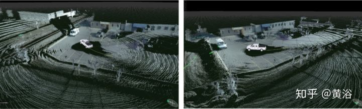
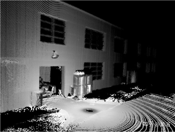
The following figure shows the point cloud results collected after calibration:
The calibration algorithm is as follows:
4 Radar - Camera Calibration
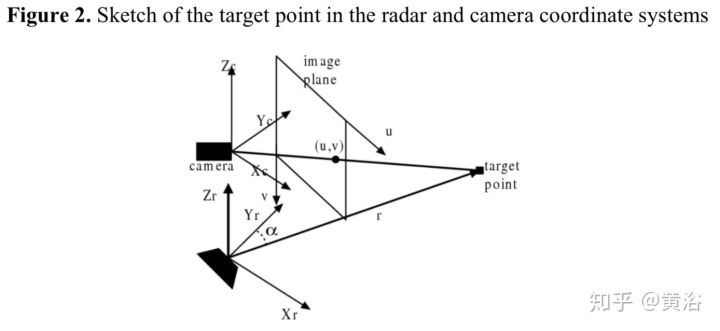
Thesis from Xi'an Jiaotong University “Integrating Millimeter Wave Radar with a Monocular Vision Sensor for On-Road Obstacle Detection Applications”。
When discussing sensor fusion, this part of the work was mentioned, and here the focus is on the calibration part. Firstly, the coordinate system relationship is as follows:
The sensor configuration is as follows:

The calibration environment is as follows:
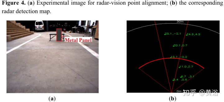
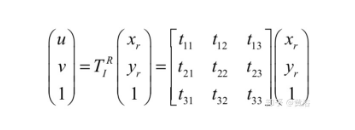
Calibration is actually calculating the homography matrix parameters between the image plane and the radar reflection surface, as shown in the following figure:
Reproduction of Zizhihu@黄浴,The viewpoints in the article are for sharing and communication only. If there are any copyright or other issues involved, please let us know and we will handle them promptly.